envMRMEGAfm: environment-adjusted MR-MEGA Fine-mapping
Siru Wang
sw2077@cam.ac.uk05 August, 2025
envMRMEGAfm.RmdIntroduction
The R package envMRMEGAfm (env-MR-MEGA fine-mapping) is designed for simultaneously fine-mapping genetic associations across multiple cohorts, allowing for multiple causal variants. This method only requires cohort-level summary statistics, the corresponding linkage disequilibrium (LD) matrices, and optionally, cohort-level environmental covariates (e.g. mean or proportion). Sometimes, we are unable to obtain LD from each cohort. In such cases, we can estimate LD structure using reference panels, such as 1000 Genomes (Consortium et al. 2015), from a genetically similar population to the GWAS. This method is powerful, versatile and computationally fast in pinpointing potential causal variants while accounting for differing environmental exposures that are specific to each cohort, in addition to ancestry.
Accounting for environmental exposures that differ between cohorts and likely impact the variability of traits, the R package envMRMEGAfm introduces MR-MEGAfm and env-MR-MEGAfm, building upon MR-MEGA (Mägi et al. 2017) and env-MR-MEGA (Wang et al. 2024) meta-regression frameworks. In addition to the two key fine-mapping methods, envMRMEGAfm package also includes the method for estimating conditional and joint genetic variant effects, which was proposed in GCTA (Yang et al. 2012) and the meta-analysis approaches, MR-MEGA (Mägi et al. 2017) and env-MR-MEGA (Wang et al. 2024).
The main R functions in this package are:
env_MR_MEGA_fm:A fine-mapping approach applicable across multiple cohorts, with the flexibility to account for both ancestral and environmental effects (env-MR-MEGAfm) or only ancestral effects (MR-MEGAfm).MR_mega_run: The (environment-adjusted) MR-MEGA meta-regression model.meta_sel_condest: The approximate conditional genetic effects method.meta_sel_joinest: The approximate joint genetic effects method.
This vignette guides readers in fine-mapping the genetic associations for a trait across multiple cohorts using MR-MEGAfm and env-MR-MEGAfm. For convenience of illustration, a simulated dataset is provided in the envMRMEGAfm package and details of how to run (env-)MR-MEGAfm method on your own data are explained.
Preparation for (env-)MR-MEGAfm
Before running the (env-)MR-MEGAfm method, several input files need to be prepared. Each input file must also include mandatory columns about genetic variants.
Input data and format requirements
The (env-)MR-MEGAfm starts with a model with the most significant SNP
in the single-SNP meta-analysis with P value below the genome-wide
significant level \(5\times 10^{-8}\).
Therefore, it is required that the single-SNP meta-analysis are
conducted by MR-MEGA (Mägi et al. 2017) and env-MR-MEGA
(Wang et al.
2024). It is noted that the meta-analysis results from both
MR-MEGA and env-MR-MEGA can be obtained from MR_mega_lrw
and MR_mega_env_lrw, which are wrapper functions in the
env.MRmega R package.
For an overview of env.MRmega R package, see env.MRmega GitHub page.
- A list of GWAS files is required for conducting both the meta-analysis and the following fine-mapping methods. The format of each file has mandatory column headers, as in the MR-MEGA software :
-
MARKERNAME- snp name -
N- sample size -
EAF- effect allele frequency -
EA- effect allele -
NEA- non effect allele -
CHROMOSOME- chromosome of marker -
POSITION- position of marker -
BETA- beta -
SE- std.error
When fitting the (env-)MR-MEGA model and running (env-)MR-MEGAfm method, we need to prepare the axes of genetic variation (PCs) and the cohort-level environment exposures. If PCs are not available,
MR_mega_MDSR function implemented in env.MRmega package is used for calculating PCs by inputting the file containing all GWAS files location and the number of PCs.The meta-analysis results, as the second required file, can be obtained from either MR-MEGA software or env.MRmega package. The output from both approaches must contain the following columns.
MARKERNAME: unique marker identification across all cohorts.CHROMOSOME: chromosome of marker.POSITION: physical position in chromosome of marker.N: sample size.chisq_association,ndf_associationandpvalue_association: test of the null hypothesis of no association of each variant.chisq_,ndf_andpvalue_refer to chisq value, number of degrees of freedom and p-values of the corresponding test.
- In addition to the list of GWAS files and the corresponding
meta-analysis results, the (env-)MR-MEGAfm method requires the
cohort-level LD correlation matrices as a third input file. When the
cohort-level LD correlation is unavailable, an approximation of the LD
correlation matrix based on a reference panel may be used. For each LD
correlation structure, both the column names and row names correspond to
MARKERNAME.
Simulation example
In this simulated data example, we considered 5 continental African populations which were collected from Phase 3 of the 1000 Genomes Project (Consortium et al. 2015). The five populationss are coded as ESN, GWD, LWK, MSL, YRI. Using the genotype data from each of the five cohorts, we used HAPGEN2 (Su, Marchini, and Donnelly 2011) software to generate individual-level genotype data of each cohort, with a sample size of 10,000 for each cohort. Within each population, we retained variants with MAF>0.01, regardless of whether the variant satisfies the MAF threshold in the other African populations. Under this setting, the number of retained variants differs across populations: 301 in ESN, 291 in GWD, 289 in LWK, 299 in MSL and 292 in YRI. Each populations is then stratified into female and male cohorts. When simulating 10 sex-stratified GWAS files for a region in chromosome19: 45711510-45770083, two randomly selected genetic variants, rs73939822 and rs60269219, were designed as causal variants (CVs) across all cohorts. Additionally, the corresponding population-level LD correlation matrices are calculated and can be loaded from the envMRMEGAfm package.
Fig 1 shows that the first two axes of genetic variation from multi-dimensional scaling of the Euclidean distance matrix between 10 sex-stratified cohorts are sufficient to separate population groups from different regions of Africa: east Africa (LWK), west-central Africa (ESN,YRI) and west Africa (GWD, MSL).
knitr::include_graphics('./figure/pcs_cnAFR.png')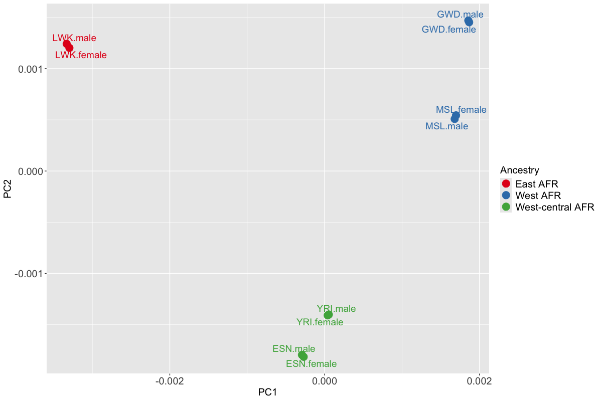
Figure 1. Axes of genetic variation separating five continental African cohorts
Accounting for sex indicators and environmental exposures which differ across all cohorts, we introduce sex and smoking status as the two environmental covariates. Cohort-level environmental covariates are constructed by taking the mean or proportion of each individual-level covariate. Cohort-level sex and smoking covariates can be loaded using the following codes:
library(envMRMEGAfm)
data(sexsmk)
sexsmk
#>    sex  smoke
#> 1    1 0.2120
#> 2    0 0.8314
#> 3    1 0.1890
#> 4    0 0.6750
#> 5    1 0.2332
#> 6    0 0.8014
#> 7    1 0.2652
#> 8    0 0.6554
#> 9    1 0.2608
#> 10   0 0.8810
For simulating the (environment-adjusted) meta-analysis results, we derived two axes of genetic variation (PCs) from a subset of variant with MAF>5% in across 10 sex-stratified African cohorts. The PCs can be loaded from envMRMEGAfm package and are shown in the following:
library(envMRMEGAfm)
data(pcs)
pcs
#>               V1           V2
#> 1  -0.0035230264 -0.027745304
#> 2  -0.0038187733 -0.027451544
#> 3   0.0243106090  0.022216813
#> 4   0.0241666027  0.022483699
#> 5  -0.0429318096  0.018390796
#> 6  -0.0433946312  0.018995055
#> 7   0.0221012729  0.008319361
#> 8   0.0218724163  0.007775967
#> 9   0.0005143428 -0.021555609
#> 10 0.0007029969 -0.021429234Note: - If PCs are not
available, MR_mega_MDS function implemented in env.MRMEGA package
is used for calculating PCs by inputting the file containing all GWAS
files location and the number of PCs.
Data pre-processing
In envMRMEGAfm package, R function
env_MR_MEGA_fm is the main tool for fine-mapping genetic
associations for the specified traits. Before performing the
fine-mapping procedure, we need to make sure that all GWAS and LD
matrices are aligned to the same reference allele. Additionally, some
large-scaled LD matrices might contain redundant variants that are not
present in all GWAS files. Through data pre-processing, we simplify the
raw LD data by removing these redundant variants.
In practice, since both GWAS files and LD matrices contain a large
amount of genetic variants information, we need to create two input
files: one for all GWAS files locations and another for LD matrices
locations. The read_gwasld function is used for
pre-processing these raw data.
gwas.loc=c("/Volumes/Mac/Stepwise_conditioning/Codes/env-MR-MEGAfm-Rpack/g1000_5afr_Rpack/gwasfile/esn_female.txt",
           "/Volumes/Mac/Stepwise_conditioning/Codes/env-MR-MEGAfm-Rpack/g1000_5afr_Rpack/gwasfile/esn_male.txt",
           "/Volumes/Mac/Stepwise_conditioning/Codes/env-MR-MEGAfm-Rpack/g1000_5afr_Rpack/gwasfile/gwd_female.txt",
           "/Volumes/Mac/Stepwise_conditioning/Codes/env-MR-MEGAfm-Rpack/g1000_5afr_Rpack/gwasfile/gwd_male.txt",
           "/Volumes/Mac/Stepwise_conditioning/Codes/env-MR-MEGAfm-Rpack/g1000_5afr_Rpack/gwasfile/lwk_female.txt",
           "/Volumes/Mac/Stepwise_conditioning/Codes/env-MR-MEGAfm-Rpack/g1000_5afr_Rpack/gwasfile/lwk_male.txt",
           "/Volumes/Mac/Stepwise_conditioning/Codes/env-MR-MEGAfm-Rpack/g1000_5afr_Rpack/gwasfile/msl_female.txt",
           "/Volumes/Mac/Stepwise_conditioning/Codes/env-MR-MEGAfm-Rpack/g1000_5afr_Rpack/gwasfile/msl_male.txt",
           "/Volumes/Mac/Stepwise_conditioning/Codes/env-MR-MEGAfm-Rpack/g1000_5afr_Rpack/gwasfile/yri_female.txt",
           "/Volumes/Mac/Stepwise_conditioning/Codes/env-MR-MEGAfm-Rpack/g1000_5afr_Rpack/gwasfile/yri_male.txt")

ld.loc=c("/Volumes/Mac/Stepwise_conditioning/Codes/env-MR-MEGAfm-Rpack/g1000_5afr_Rpack/LD/esn.txt",
         "/Volumes/Mac/Stepwise_conditioning/Codes/env-MR-MEGAfm-Rpack/g1000_5afr_Rpack/LD/gwd.txt",
         "/Volumes/Mac/Stepwise_conditioning/Codes/env-MR-MEGAfm-Rpack/g1000_5afr_Rpack/LD/lwk.txt",
         "/Volumes/Mac/Stepwise_conditioning/Codes/env-MR-MEGAfm-Rpack/g1000_5afr_Rpack/LD/msl.txt",
         "/Volumes/Mac/Stepwise_conditioning/Codes/env-MR-MEGAfm-Rpack/g1000_5afr_Rpack/LD/yri.txt")

LD=c("esn","gwd","lwk","msl","yri")
#Each African population is stratified into male and female cohorts.
pop=c("esn.female","esn.male","gwd.female","gwd.male","lwk.female","lwk.male","msl.female","msl.male","yri.female","yri.male")

gwasld=read_gwasld(gwas.loc,ld.loc,which.ld=rep(LD,each=2),cohort_name=pop,ld_name=LD,out_loc=NULL)
#> [1] "i in filesize 1"
#> [1] "Reading gwas file /Volumes/Mac/Stepwise_conditioning/Codes/env-MR-MEGAfm-Rpack/g1000_5afr_Rpack/gwasfile/esn_female.txt"
#> There are  301  SNPs in this GWAS file
#> [1] "i in filesize 2"
#> [1] "Reading gwas file /Volumes/Mac/Stepwise_conditioning/Codes/env-MR-MEGAfm-Rpack/g1000_5afr_Rpack/gwasfile/esn_male.txt"
#> There are  301  SNPs in this GWAS file
#> [1] "i in filesize 3"
#> [1] "Reading gwas file /Volumes/Mac/Stepwise_conditioning/Codes/env-MR-MEGAfm-Rpack/g1000_5afr_Rpack/gwasfile/gwd_female.txt"
#> There are  291  SNPs in this GWAS file
#> [1] "i in filesize 4"
#> [1] "Reading gwas file /Volumes/Mac/Stepwise_conditioning/Codes/env-MR-MEGAfm-Rpack/g1000_5afr_Rpack/gwasfile/gwd_male.txt"
#> There are  291  SNPs in this GWAS file
#> [1] "i in filesize 5"
#> [1] "Reading gwas file /Volumes/Mac/Stepwise_conditioning/Codes/env-MR-MEGAfm-Rpack/g1000_5afr_Rpack/gwasfile/lwk_female.txt"
#> There are  289  SNPs in this GWAS file
#> [1] "i in filesize 6"
#> [1] "Reading gwas file /Volumes/Mac/Stepwise_conditioning/Codes/env-MR-MEGAfm-Rpack/g1000_5afr_Rpack/gwasfile/lwk_male.txt"
#> There are  289  SNPs in this GWAS file
#> [1] "i in filesize 7"
#> [1] "Reading gwas file /Volumes/Mac/Stepwise_conditioning/Codes/env-MR-MEGAfm-Rpack/g1000_5afr_Rpack/gwasfile/msl_female.txt"
#> There are  299  SNPs in this GWAS file
#> [1] "i in filesize 8"
#> [1] "Reading gwas file /Volumes/Mac/Stepwise_conditioning/Codes/env-MR-MEGAfm-Rpack/g1000_5afr_Rpack/gwasfile/msl_male.txt"
#> There are  299  SNPs in this GWAS file
#> [1] "i in filesize 9"
#> [1] "Reading gwas file /Volumes/Mac/Stepwise_conditioning/Codes/env-MR-MEGAfm-Rpack/g1000_5afr_Rpack/gwasfile/yri_female.txt"
#> There are  292  SNPs in this GWAS file
#> [1] "i in filesize 10"
#> [1] "Reading gwas file /Volumes/Mac/Stepwise_conditioning/Codes/env-MR-MEGAfm-Rpack/g1000_5afr_Rpack/gwasfile/yri_male.txt"
#> There are  294  SNPs in this GWAS file
#> [1] "i in filesize 1"
#> [1] "Reading LD file /Volumes/Mac/Stepwise_conditioning/Codes/env-MR-MEGAfm-Rpack/g1000_5afr_Rpack/LD/esn.txt"
#> [1] 301 301
#> [1] "i in filesize 2"
#> [1] "Reading LD file /Volumes/Mac/Stepwise_conditioning/Codes/env-MR-MEGAfm-Rpack/g1000_5afr_Rpack/LD/gwd.txt"
#> [1] 291 291
#> [1] "i in filesize 3"
#> [1] "Reading LD file /Volumes/Mac/Stepwise_conditioning/Codes/env-MR-MEGAfm-Rpack/g1000_5afr_Rpack/LD/lwk.txt"
#> [1] 289 289
#> [1] "i in filesize 4"
#> [1] "Reading LD file /Volumes/Mac/Stepwise_conditioning/Codes/env-MR-MEGAfm-Rpack/g1000_5afr_Rpack/LD/msl.txt"
#> [1] 299 299
#> [1] "i in filesize 5"
#> [1] "Reading LD file /Volumes/Mac/Stepwise_conditioning/Codes/env-MR-MEGAfm-Rpack/g1000_5afr_Rpack/LD/yri.txt"
#> [1] 293 293
#> [1] "Assign each GWAS file to the corresponding LD structure......"
#> [1] "matrix" "array"
#> [1] 301 301
#> [1] "matrix" "array"
#> [1] 291 291
#> [1] "matrix" "array"
#> [1] 289 289
#> [1] "matrix" "array"
#> [1] 299 299
#> [1] "matrix" "array"
#> [1] 293 293
gwas.list=gwasld$gwas.list

ld.list=gwasld$ld.list
In the commands above, read_gwasld function outputs two
files: one containing the pre-processed GWAS files and another
containing the pre-processed LD matrices. These pre-processed GWAS files
and LD matrices can be loaded from the envMRMEGAfm
package.
More specifically, the above arguments present in
read_gwasld function are:
gwas.loc: A file contains a vector of length \(K_g\). Each component of the vector refers to the location of GWAS file.ld.loc: A file contains a vector of length \(K_{ld}\). Each component of the vector refers to the location of LD structure files.which.ld: A character vector of length \(K_g\). Each component of the vector corresponds to one LD structure. The length of which.ld should equal to the number of GWAS files. Note: the argumentwhich.ldis regarded as a link between GWAS files and LD files. Each component ofwhich.ldvector results from one of the LD names.cohort_name: A character vector of length \(K_g\). Each component of the vector corresponds to one GWAS file.ld_name: A character vector of length \(K_{ld}\). Each component of the vector corresponds to one LD structure.out_loc: Path to save pre-processed GWAS files and LD structure. By default,out_loc=NULL.actual.geno: An indicator to specify whether the true cohort-level LD structure is provided. If we can obtain the real cohort-level LD structures directly or derive LD structures from the real individual-level genotype data of the involved cohorts, the argumentactual.genois set toTRUE. If we estimate LD approximation from the reference sample as a replacement,actual.genois set toFALSE. By defaultactual.geno=FALSE.The default value is consistent for GCTA-COJO setting.
Fine-mapping
In the simulation design where the allelic heterogeneity is
correlated with smoking status, we applied env-MR-MEGAfm method and
MR-MEGAfm to the simulated example respectively. Different from
env-MR-MEGAfm, we run MR-MEGAfm by setting the argument env
as NULL. In addition to some arguments appearing in
read_gwasld function, there are other arguments in
env_MR_MEGA_fm function. The additional arguments are
illustrated in the following:
meta.file: The meta-analysis results obtained from the output of MR-MEGA method or env-MR-MEGA method. A dataframe contains some mandatory columns where Preparation for (env-)MR-MEGAfm section gives the further details.ncores: The number of cores which would be used for running in parallel.collinear: A correlation threshold to filter out the target SNP in high LD with the SNP set. If the squared multiple correlation between the target SNP exceeds the threshold, such as 0.9, the target SNP is ignored.pvalue_cutoff: A p-value threshold to identify genetic associations. By default,pvalue_cutoff=5e-8.cred.thr: Credible threshold for the credible set for each selected potential SNP. By default,cred.thr=0.99 refers to 99% credible sets.
Note:
In this simulated example, LD correlation matrix of each population was derived from the true individual-level genotype data, with the argument
actual.genoset toTRUE. However, in some cases, individual-level genotype data for each cohort are poor, resulting in unavailable for calculation of LD matrices. In such cases, the LD matrix can be estimated using a reference panel (e.g. 1000 Genomes) from a genetically similar population to the samples used for genotype-phenotype association analysis. When the approximation of LD matrix is applied, argumentactual.genoshould be set toFALSE.For (env-)MR-MEGAfm method, the key model selection strategy is built upon (env-)MR-MEGA meta-analysis framework. As a result, (env-)MR-MEGAfm method has the limitations regarding the number of PCs (T) and the number of environment exposures (K). Specifically, for MR-MEGAfm, across (K) cohorts, the number of axes of genetic variation (T) is constrained by T<K-2. For env-MR-MEGAfm, the limitation extends to the sum of the number of axes of genetic variation (T) and the number of environmental covariates (S), with the limitation T+S<K-2.
env-MR-MEGAfm
names(gwas.list)
#>  [1] "esn.female" "esn.male"   "gwd.female" "gwd.male"   "lwk.female"
#>  [6] "lwk.male"   "msl.female" "msl.male"   "yri.female" "yri.male"
names(ld.list)
#> [1] "esn" "gwd" "lwk" "msl" "yri"
######################################env-MR-MEGA fine-mapping###################################
tictoc::tic("Run env-MR-MEGA fine-mapping method")
library(doParallel)
#> Loading required package: foreach
#> Loading required package: iterators
#> Loading required package: parallel
envmetafm.out=env_MR_MEGA_fm(gwas.list,ld.list,which.ld=rep(names(ld.list),each=2),meta.file=envMRMEGAout,PCs=pcs,env=sexsmk,out_loc=NULL,ncores=2,collinear=0.9,pvalue_cutoff=5e-8,cred.thr=0.99)
#> (Collinearity cutoff =  0.9 )
#> The number of cores are  2 , which are used for running in parallel
#> The threshold for credible set is set to  0.99 .
#> i.pop is  1
#> Whether the inputted LD is cohort-matched LD FALSE
#> i.pop is  2
#> Whether the inputted LD is cohort-matched LD FALSE
#> i.pop is  3
#> Whether the inputted LD is cohort-matched LD FALSE
#> i.pop is  4
#> Whether the inputted LD is cohort-matched LD FALSE
#> i.pop is  5
#> Whether the inputted LD is cohort-matched LD FALSE
#> i.pop is  6
#> Whether the inputted LD is cohort-matched LD FALSE
#> i.pop is  7
#> Whether the inputted LD is cohort-matched LD FALSE
#> i.pop is  8
#> Whether the inputted LD is cohort-matched LD FALSE
#> i.pop is  9
#> Whether the inputted LD is cohort-matched LD FALSE
#> i.pop is  10
#> Whether the inputted LD is cohort-matched LD FALSE
#> At the  1 iteration, the set of the selected SNPs include
#> [1] "rs73939822"
#> [1] "All GWAS are assigned to the same reference allele"
#> [1] "At the same, the correponding LD structures should be adjusted accordingly."
#> At the  2 iteration, the set of the selected SNPs include
#> [1] "rs73939822" "rs60269219"
#> The target selected genetic variant is rs73939822
#> [1] "All GWAS are assigned to the same reference allele"
#> [1] "At the same, the correponding LD structures should be adjusted accordingly."
#> The target selected genetic variant is rs60269219
#> [1] "All GWAS are assigned to the same reference allele"
#> [1] "At the same, the correponding LD structures should be adjusted accordingly."
#> [1] "All GWAS are assigned to the same reference allele"
#> [1] "At the same, the correponding LD structures should be adjusted accordingly."
#> There are  2  potential associated SNPs!
#> The target selected genetic variant is rs73939822
#> [1] "All GWAS are assigned to the same reference allele"
#> [1] "At the same, the correponding LD structures should be adjusted accordingly."
#> The target selected genetic variant is rs60269219
#> [1] "All GWAS are assigned to the same reference allele"
#> [1] "At the same, the correponding LD structures should be adjusted accordingly."
tictoc::toc()
#> Run env-MR-MEGA fine-mapping method: 22.575 sec elapsed
envmetafm.out
#> $sel.set
#> [1] "rs73939822" "rs60269219"
#>
#> $tgCS.thr
#> $tgCS.thr$rs73939822
#>     MARKERNAME chisq_association ndf_association pvalue_association
#> 215 rs73939822          1972.823               5                  0
#>     chisq_anc_env_het ndf_chisq_anc_env_het pvalue_anc_env_het chisq_residual
#> 215          424.8579                     4       1.181767e-90       6.102112
#>     ndf_residual pvalue_residual   logBF chisq_env_het ndf_env_het
#> 215            5       0.2964094 980.655      413.6669           2
#>     pvalue_env_het chisq_anc_het ndf_anc_het pvalue_anc_het       PPs maxld
#> 215   1.490651e-90      2.552803           2      0.2790396 0.9987435     1
#>     cs.inc
#> 215      1
#>
#> $tgCS.thr$rs60269219
#>    MARKERNAME chisq_association ndf_association pvalue_association
#> 77 rs60269219          1701.090               5                  0
#> 76 rs61079153          1699.642               5                  0
#> 78 rs59356929          1691.853               5                  0
#>    chisq_anc_env_het ndf_chisq_anc_env_het pvalue_anc_env_het chisq_residual
#> 77          437.7434                     4       1.938165e-93       5.764427
#> 76          437.3153                     4       2.398521e-93       5.911945
#> 78          432.7377                     4       2.341041e-92       5.978292
#>    ndf_residual pvalue_residual    logBF chisq_env_het ndf_env_het
#> 77            5       0.3298202 844.7887      426.7314           2
#> 76            5       0.3148816 844.0645      426.5248           2
#> 78            5       0.3083369 840.1698      421.8789           2
#>    pvalue_env_het chisq_anc_het ndf_anc_het pvalue_anc_het         PPs maxld
#> 77   2.169937e-93      6.716531           2     0.03479557 0.666173442     1
#> 76   2.406172e-93      6.681750           2     0.03540597 0.322890947     1
#> 78   2.455613e-92      6.643331           2     0.03609267 0.006570714     1
#>    cs.inc
#> 77      1
#> 76      1
#> 78      1
MR-MEGAfm
######################################MR-MEGA fine-mapping###################################
tictoc::tic("Run env-MR-MEGA fine-mapping method")
library(doParallel)
metafm.out=env_MR_MEGA_fm(gwas.list,ld.list,which.ld=rep(names(ld.list),each=2),meta.file=MRMEGAout,PCs=pcs,env=NULL,out_loc=NULL,ncores=2,collinear=0.9,pvalue_cutoff=5e-8,cred.thr=0.99)
#> (Collinearity cutoff =  0.9 )
#> The number of cores are  2 , which are used for running in parallel
#> The threshold for credible set is set to  0.99 .
#> i.pop is  1
#> Whether the inputted LD is cohort-matched LD FALSE
#> i.pop is  2
#> Whether the inputted LD is cohort-matched LD FALSE
#> i.pop is  3
#> Whether the inputted LD is cohort-matched LD FALSE
#> i.pop is  4
#> Whether the inputted LD is cohort-matched LD FALSE
#> i.pop is  5
#> Whether the inputted LD is cohort-matched LD FALSE
#> i.pop is  6
#> Whether the inputted LD is cohort-matched LD FALSE
#> i.pop is  7
#> Whether the inputted LD is cohort-matched LD FALSE
#> i.pop is  8
#> Whether the inputted LD is cohort-matched LD FALSE
#> i.pop is  9
#> Whether the inputted LD is cohort-matched LD FALSE
#> i.pop is  10
#> Whether the inputted LD is cohort-matched LD FALSE
#> At the  1 iteration, the set of the selected SNPs include
#> [1] "rs73939822"
#> [1] "All GWAS are assigned to the same reference allele"
#> [1] "At the same, the correponding LD structures should be adjusted accordingly."
#> At the  2 iteration, the set of the selected SNPs include
#> [1] "rs73939822" "rs60269219"
#> The target selected genetic variant is rs73939822
#> [1] "All GWAS are assigned to the same reference allele"
#> [1] "At the same, the correponding LD structures should be adjusted accordingly."
#> The target selected genetic variant is rs60269219
#> [1] "All GWAS are assigned to the same reference allele"
#> [1] "At the same, the correponding LD structures should be adjusted accordingly."
#> [1] "All GWAS are assigned to the same reference allele"
#> [1] "At the same, the correponding LD structures should be adjusted accordingly."
#> There are  2  potential associated SNPs!
#> The target selected genetic variant is rs73939822
#> [1] "All GWAS are assigned to the same reference allele"
#> [1] "At the same, the correponding LD structures should be adjusted accordingly."
#> The target selected genetic variant is rs60269219
#> [1] "All GWAS are assigned to the same reference allele"
#> [1] "At the same, the correponding LD structures should be adjusted accordingly."
tictoc::toc()
#> Run env-MR-MEGA fine-mapping method: 20.796 sec elapsed
metafm.out
#> $sel.set
#> [1] "rs73939822" "rs60269219"
#>
#> $tgCS.thr
#> $tgCS.thr$rs73939822
#>      MARKERNAME chisq_association ndf_association pvalue_association
#> 215  rs73939822          1559.156               3                  0
#> 222 rs143024846          1551.294               3                  0
#>     chisq_anc_het ndf_chisq_anc_het pvalue_anc_het chisq_residual ndf_residual
#> 215      11.19101                 2    0.003714517       419.7690            7
#> 222      10.05222                 2    0.006564303       414.2482            7
#>     pvalue_residual    logBF        PPs maxld cs.inc
#> 215    1.370481e-86 776.1242 0.98075059     1      1
#> 222    2.096064e-85 772.1933 0.01924941     1      1
#>
#> $tgCS.thr$rs60269219
#>    MARKERNAME chisq_association ndf_association pvalue_association
#> 77 rs60269219          1274.359               3      5.387582e-276
#> 76 rs61079153          1273.117               3      1.001923e-275
#> 78 rs59356929          1269.974               3      4.818463e-275
#> 82 rs57294488          1268.921               3      8.154631e-275
#>    chisq_anc_het ndf_chisq_anc_het pvalue_anc_het chisq_residual ndf_residual
#> 77      11.01200                 2    0.004062321       432.4959            7
#> 76      10.79051                 2    0.004538063       432.4367            7
#> 78      10.85875                 2    0.004385831       427.8572            7
#> 82      10.98314                 2    0.004121372       428.0893            7
#>    pvalue_residual    logBF        PPs maxld cs.inc
#> 77    2.544181e-89 633.7256 0.58308761     1      1
#> 76    2.619670e-89 633.1047 0.31338763     1      1
#> 78    2.518646e-88 631.5329 0.06508363     1      1
#> 82    2.245652e-88 631.0064 0.03844113     1      1
The results from both MR-MEGAfm and env-MR-MEGAfm comprise two main parts:
sel.set: The selected potential associated SNP set.tgCS.thr: A list of the credible sets of the selected SNPs under the specified threshold. By default, the specified threshold is set to 0.99. Each component of the list is a dataframe containing the following columns:MARKERNAME: unique marker identification across all cohorts.chisq_association,ndf_associationandpvalue_association: test of the null hypothesis of no association of each variant.chisq_,ndf_andpvalue_refer to chisq value, number of degrees of freedom and p-values of the corresponding test.chisq_residual,ndf_residualandpvalue_residual: test of residual heterogeneity.logBF: log of Bayesian Factor.PPs: Posterior probability.max_ld: The maximum of LD value between each target selected variant and the variants in the credible set.cs.inc: The indicator for determining whether the variants should be included in the credible sets based on the specified credible threshold.
For MR-MEGAfm,
-
chisq_anc_het,ndf_anc_hetandpvalue_anc_het: test of ancestral heterogeneity.
For env-MR-MEGAfm, results contain tests which are different from MR-MEGAfm.
chisq_anc_env_het,ndf_anc_env_hetandpvalue_anc_env_het: test of ancestral and environmental heterogeneity.chisq_anc_het,ndf_anc_hetandpvalue_anc_het: test of allelic heterogeneity due to ancestry alone.chisq_env_het,ndf_env_hetandpvalue_env_het: test of allelic heterogeneity due to environment alone.