env.MRmega
Siru Wang
sw2077@cam.ac.uk17 November, 2024
Source:vignettes/envMRmega.Rmd
envMRmega.RmdIntroduction
env.MRmega (Environment-adjusted MR-MEGA) is a package to identify genetic variants that are associated with each trait, across cohorts, while adjusting for differing environmental exposures between cohorts. For the environment-adjusted MR-MEGA approach, we will adapt the original MR-MEGA meta-regression framework to account for environmental exposures that are specific each cohort. Apart from environment-adjusted MR-MEGA methodology, the R package also includes pre-processing of the inputted GWAS files, calculation of axes of genetic variation and the original MR-MEGA methodology.
This vignette introduces the whole meta-analysis procedure using the original MR-MEGA approach and the environment-adjusted MR-MEGA approach.
GWAS data format
No matter which meta-analysis methods (environment-adjusted MR-MEGA or MR-MEGA) are applied, a list of GWAS datasets would be the main input as required, and each GWAS data must contain mandatory columns. Details of GWAS format would be given by a simple simulation.
For convenience of illustration, we would grossly simulate several GWAS datasets containing medium-sized genetic variants and the associated genetic information. In the simulated data, we considered 7 sub-populations of African ancestry which were collected from Phase 3 of the 1000 Genomes Project(Consortium et al. 2015),see https://ctg.cncr.nl/software/MAGMA/ref_data/. The 7 populations were coded as ACB, ASW, ESN, GWD, LWK, MSL, YRI. Among the 7 GWAS raw data, we randomly selected 50 genetic variants across 23 chromosomes to create 7 medium-sized GWAS files. The format of each file has mandatory column headers, shown as MR-MEGA software (https://genomics.ut.ee/en/tools):
-
MARKERNAME- snp name -
N- sample size -
EAF- effect allele frequency -
EA- effect allele -
NEA- non effect allele -
CHROMOSOME- chromosome of marker -
POSITION- position of marker -
BETA- beta -
SE- std.error
When simulating quantitative traits, in the specified African
populations (ESN, GWD,
LWK), we consider equal-sized populations (4K in each
population). Then we set three genetic
variants,rs201029612, rs79862059 and
rs77833422, which are associated with the quantitative
traits. To mimic the real GWAS data in which some genetic variants would
not exist in all populations, we made that the two genetic variants,
rs190897515 and rs577430535, exist in
ACB population only; one genetic variant
rs185581532 exists in 5 populations only and one genetic
variant rs572565163 exists in 4 populations only. The
details of 7 simulated GWAS data are saved in afr.gwas
object as a list.
require(env.MRmega)
#> Loading required package: env.MRmega
lapply(afr.gwas,function(x){head(x,2)})
#> $acb
#>     MARKERNAME     N    EAF      BETA       SE CHROMOSOME POSITION     EA
#>         <char> <int>  <num>     <num>    <num>      <int>    <int> <char>
#> 1:  rs10429359  4000 0.3646 -0.000422 0.010527          8 72918699      C
#> 2: rs115995911  4000 0.1042 -0.001478 0.016606         10 73624098      T
#>       NEA
#>    <char>
#> 1:      G
#> 2:      C
#>
#> $asw
#>     MARKERNAME     N    EAF      BETA       SE CHROMOSOME POSITION     EA
#>         <char> <int>  <num>     <num>    <num>      <int>    <int> <char>
#> 1:  rs10429359  4000 0.3115 -0.018387 0.010747          8 72918699      C
#> 2: rs115995911  4000 0.1885 -0.005697 0.012782         10 73624098      T
#>       NEA
#>    <char>
#> 1:      G
#> 2:      C
#>
#> $esn
#>     MARKERNAME     N    EAF      BETA       SE CHROMOSOME POSITION     EA
#>         <char> <int>  <num>     <num>    <num>      <int>    <int> <char>
#> 1:  rs10429359  4000 0.3283  0.000632 0.010673          8 72918699      C
#> 2: rs115995911  4000 0.1515 -0.023159 0.014028         10 73624098      T
#>       NEA
#>    <char>
#> 1:      G
#> 2:      C
#>
#> $gwd
#>     MARKERNAME     N    EAF      BETA       SE CHROMOSOME POSITION     EA
#>         <char> <int>  <num>     <num>    <num>      <int>    <int> <char>
#> 1:  rs10429359  4000 0.3805  0.012997 0.010300          8 72918699      C
#> 2: rs115995911  4000 0.2212 -0.026722 0.012143         10 73624098      T
#>       NEA
#>    <char>
#> 1:      G
#> 2:      C
#>
#> $lwk
#>     MARKERNAME     N     EAF     BETA       SE CHROMOSOME POSITION     EA
#>         <char> <int>   <num>    <num>    <num>      <int>    <int> <char>
#> 1:  rs10429359  4000 0.30810 0.021422 0.010870          8 72918699      C
#> 2: rs115995911  4000 0.07071 0.000319 0.020456         10 73624098      T
#>       NEA
#>    <char>
#> 1:      G
#> 2:      C
#>
#> $msl
#>     MARKERNAME     N    EAF      BETA       SE CHROMOSOME POSITION     EA
#>         <char> <int>  <num>     <num>    <num>      <int>    <int> <char>
#> 1:  rs10429359  4000 0.3118 -0.011872 0.010834          8 72918699      C
#> 2: rs115995911  4000 0.1647  0.015265 0.013528         10 73624098      T
#>       NEA
#>    <char>
#> 1:      G
#> 2:      C
#>
#> $yri
#>     MARKERNAME     N    EAF      BETA       SE CHROMOSOME POSITION     EA
#>         <char> <int>  <num>     <num>    <num>      <int>    <int> <char>
#> 1:  rs10429359  4000 0.3935  0.016963 0.010342          8 72918699      C
#> 2: rs115995911  4000 0.1898 -0.009583 0.012878         10 73624098      T
#>       NEA
#>    <char>
#> 1:      G
#> 2:      C
In real life, GWAS statistic data of each cohort would be saved as a
file (“.txt”), even a compressed file (“.txt.gz”), containing tens of
thousands of genetic variants information. We could create a input file
which contains all study files and use readInputfile
function to aggregate several GWAS files into a list.
data_name=c("~/Desktop/mr-mega-r/MR_MEGA_ENV_git/g1000_afr_7gwas_git/afr_acb_EGL20.txt",
            "~/Desktop/mr-mega-r/MR_MEGA_ENV_git/g1000_afr_7gwas_git/afr_asw_EGL20.txt",
            "~/Desktop/mr-mega-r/MR_MEGA_ENV_git/g1000_afr_7gwas_git/afr_esn_EGL20.txt",
            "~/Desktop/mr-mega-r/MR_MEGA_ENV_git/g1000_afr_7gwas_git/afr_gwd_EGL20.txt",
            "~/Desktop/mr-mega-r/MR_MEGA_ENV_git/g1000_afr_7gwas_git/afr_lwk_EGL20.txt",
            "~/Desktop/mr-mega-r/MR_MEGA_ENV_git/g1000_afr_7gwas_git/afr_msl_EGL20.txt",
            "~/Desktop/mr-mega-r/MR_MEGA_ENV_git/g1000_afr_7gwas_git/afr_yri_EGL20.txt")

out<-readInputfile(data_name,qt=TRUE)
#> [1] "i in filesize 1"
#> [1] "Reading file ~/Desktop/mr-mega-r/MR_MEGA_ENV_git/g1000_afr_7gwas_git/afr_acb_EGL20.txt"
#> [1] "i in filesize 2"
#> [1] "Reading file ~/Desktop/mr-mega-r/MR_MEGA_ENV_git/g1000_afr_7gwas_git/afr_asw_EGL20.txt"
#> [1] "i in filesize 3"
#> [1] "Reading file ~/Desktop/mr-mega-r/MR_MEGA_ENV_git/g1000_afr_7gwas_git/afr_esn_EGL20.txt"
#> [1] "i in filesize 4"
#> [1] "Reading file ~/Desktop/mr-mega-r/MR_MEGA_ENV_git/g1000_afr_7gwas_git/afr_gwd_EGL20.txt"
#> [1] "i in filesize 5"
#> [1] "Reading file ~/Desktop/mr-mega-r/MR_MEGA_ENV_git/g1000_afr_7gwas_git/afr_lwk_EGL20.txt"
#> [1] "i in filesize 6"
#> [1] "Reading file ~/Desktop/mr-mega-r/MR_MEGA_ENV_git/g1000_afr_7gwas_git/afr_msl_EGL20.txt"
#> [1] "i in filesize 7"
#> [1] "Reading file ~/Desktop/mr-mega-r/MR_MEGA_ENV_git/g1000_afr_7gwas_git/afr_yri_EGL20.txt"
lapply(out,function(x){head(x,2)})
#> $Pop1
#>     MARKERNAME CHROMOSOME POSITION     EA    NEA    EAF      BETA       SE
#>         <char>      <int>    <int> <char> <char>  <num>     <num>    <num>
#> 1:  rs10429359          8 72918699      C      G 0.3646 -0.000422 0.010527
#> 2: rs115995911         10 73624098      T      C 0.1042 -0.001478 0.016606
#>        N
#>    <int>
#> 1:  4000
#> 2:  4000
#>
#> $Pop2
#>     MARKERNAME CHROMOSOME POSITION     EA    NEA    EAF      BETA       SE
#>         <char>      <int>    <int> <char> <char>  <num>     <num>    <num>
#> 1:  rs10429359          8 72918699      C      G 0.3115 -0.018387 0.010747
#> 2: rs115995911         10 73624098      T      C 0.1885 -0.005697 0.012782
#>        N
#>    <int>
#> 1:  4000
#> 2:  4000
#>
#> $Pop3
#>     MARKERNAME CHROMOSOME POSITION     EA    NEA    EAF      BETA       SE
#>         <char>      <int>    <int> <char> <char>  <num>     <num>    <num>
#> 1:  rs10429359          8 72918699      C      G 0.3283  0.000632 0.010673
#> 2: rs115995911         10 73624098      T      C 0.1515 -0.023159 0.014028
#>        N
#>    <int>
#> 1:  4000
#> 2:  4000
#>
#> $Pop4
#>     MARKERNAME CHROMOSOME POSITION     EA    NEA    EAF      BETA       SE
#>         <char>      <int>    <int> <char> <char>  <num>     <num>    <num>
#> 1:  rs10429359          8 72918699      C      G 0.3805  0.012997 0.010300
#> 2: rs115995911         10 73624098      T      C 0.2212 -0.026722 0.012143
#>        N
#>    <int>
#> 1:  4000
#> 2:  4000
#>
#> $Pop5
#>     MARKERNAME CHROMOSOME POSITION     EA    NEA     EAF     BETA       SE
#>         <char>      <int>    <int> <char> <char>   <num>    <num>    <num>
#> 1:  rs10429359          8 72918699      C      G 0.30810 0.021422 0.010870
#> 2: rs115995911         10 73624098      T      C 0.07071 0.000319 0.020456
#>        N
#>    <int>
#> 1:  4000
#> 2:  4000
#>
#> $Pop6
#>     MARKERNAME CHROMOSOME POSITION     EA    NEA    EAF      BETA       SE
#>         <char>      <int>    <int> <char> <char>  <num>     <num>    <num>
#> 1:  rs10429359          8 72918699      C      G 0.3118 -0.011872 0.010834
#> 2: rs115995911         10 73624098      T      C 0.1647  0.015265 0.013528
#>        N
#>    <int>
#> 1:  4000
#> 2:  4000
#>
#> $Pop7
#>     MARKERNAME CHROMOSOME POSITION     EA    NEA    EAF      BETA       SE
#>         <char>      <int>    <int> <char> <char>  <num>     <num>    <num>
#> 1:  rs10429359          8 72918699      C      G 0.3935  0.016963 0.010342
#> 2: rs115995911         10 73624098      T      C 0.1898 -0.009583 0.012878
#>        N
#>    <int>
#> 1:  4000
#> 2: 4000Note:
- For convenience of simplicity, we do not take account of sex stratification in this case. In real life, each GWAS file can be stratified by sex into male and female cohorts. The 7 GWAS files then would be divided into 14 cohorts, then the environment-adjusted MR-MEGA and the original MR-MEGA approaches can also be used for sex-stratified GWAS data.
For the environment-adjusted meta-regression analysis, besides the above mentioned mandatory columns in each GWAS study file, we also need to add cohort-specific environmental exposure information. Here we assume a binary environmental exposure, smoking status (1/0). Within each cohort, smoking status=1 for individuals having smoking habits and smoking status=0 for individuals having no smoking habits.
Note:
- For 14 sex-stratified cohorts, the individual-level data for environment covariates would comprise one binary smoking status and one binary sex indicator (female=1/male=0). With each sex-stratified cohort, sex indicator =1 for all female cohorts and sex indicator =0 for all male cohorts.
Simulation example
Packages installation and loading
First, we load the packages necessary for analysis, and check the version of each package.The provided demo runs in less than 2 seconds including preparation and execution of both MR-MEGA/environment-adjusted MR-MEGA procedures.
Data pre-processing
Calculate PCs
Before fitting the environment-adjusted meta-regression model and the original meta-regression model (Mägi et al. 2017), we need to specify the number of PCs (T), default=2. Specifically, we used a subset of genetic variants with MAF>5% in all population files to derive Euclidean distances matrix. Then the two axes of genetic variation were derived from the multi-dimensional scaling of the distance matrix in the corresponding reference panel. Figure 1 shows that the first two axes of genetic variation from multi-dimensional scaling of the Euclidean distance matrix between 7 populations are sufficient to separate population groups from different regions of Africa.
knitr::include_graphics('./figure/pcs_sim1.png')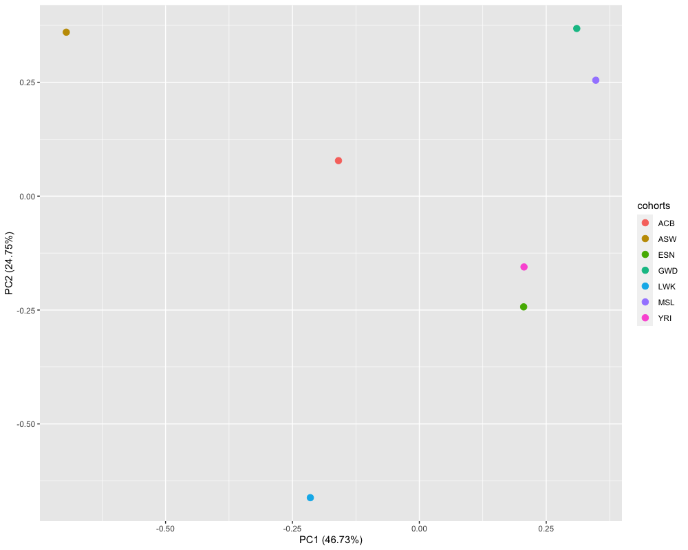
Figure 1. Axes of genetic variation separating seven populations from African ancestry
Note: the number of axes of genetic variation and the number of environmental covariates would depend on the diversity of cohorts, but the limitation of the number of axes of genetic variation (T) and the number of environmental covariates (S) should be less than the number of cohorts (K) - 2.
The function used for calculating PCs would be built in the function
MR_mega_prep which is used for preparing inputted data in
the environment-adjusted meta-regression and the original
meta-regression models. For convenience of PC calculation independently,
we extracted the function used for calculating PCs
MR_mega_MDS out. Since the simulated GWAS data contain 50
genetic variants only, we would derive PCs from the subset of genetic
variants with MAF>5% in the whole of the 7 GWAS raw files, each file
consisting of thousands of genetic variants across 23 chromosomes.
For running MR_mega_MDS function, you can create a
vector containing all population file names and the corresponding
locations. Then you need to point out the location of the output, named
by batch_loc.
Note: The data are pre-loaded and these lines should not be run in the demo.
data_name=c("~/MR_MEGA/MR_MEGA_ENV_gitdta/g1000_afr_acb/g1000_afr_acb.inf",
            "~/MR_MEGA/MR_MEGA_ENV_gitdta/g1000_afr_asw/g1000_afr_asw.inf",
            "~/MR_MEGA/MR_MEGA_ENV_gitdta/g1000_afr_esn/g1000_afr_esn.inf",
            "~/MR_MEGA/MR_MEGA_ENV_gitdta/g1000_afr_gwd/g1000_afr_gwd.inf",
            "~/MR_MEGA/MR_MEGA_ENV_gitdta/g1000_afr_lwk/g1000_afr_lwk.inf",
            "~/MR_MEGA/MR_MEGA_ENV_gitdta/g1000_afr_msl/g1000_afr_msl.inf",
            "~/MR_MEGA/MR_MEGA_ENV_gitdta/g1000_afr_yri/g1000_afr_yri.inf")
batch_loc="~/MR_MEGA/MR_MEGA_ENV_gitdta/"
MR_mega_MDS(data_name,batch_loc,qt=TRUE,pcCount=2,ncores=10)
In the above command, MR_mega_MDS function would output
two files, one file containing axes of genetic variants and another
containing multi-dimensional scaling (MDS) of Euclidean distances
matrix. After inputting 7 GWAS files, we get the PCs shown as
follows.
pcs
#>            pc1          pc2
#>          <num>        <num>
#> 1: -0.01143282  0.004831679
#> 2: -0.04685165  0.020099247
#> 3:  0.01282844 -0.012446795
#> 4:  0.02037034  0.020354682
#> 5: -0.01215912 -0.040216803
#> 6:  0.02405165  0.014331996
#> 7:  0.01319316 -0.006954006
Categorize BETA, SE and other genetic variant information into different objects
Based on the 7 simulated GWAS files, we categorized BETA
and SE into two objects which would be saved as a list via
MR_mega_prep function.
Note:
It is required that the order of names of
afr.gwasshould always be consistent with the order ofdata_nameas input inMR_mega_MDSfunction.Considering GWAS files might contain thousands of genetic variants in real life, we can also divide
BETAobject andSEobject into several batches. When conducting the environment-adjusted MR-MEGA approach and the original MR-MEGA approach, we could input these batches into the associated functions and performing them in parallel.
################env_adjusted MR-MEGA#####################
tictoc::tic("Preparation for performing MR-MEGA/env-MR-MEGA approach")
gwas_input<-MR_mega_prep(sum_stat_pop=afr.gwas,n_cohort=7,usefor="env-mr-mega",qt=TRUE,pcCount=2,calpc=FALSE,envCount=1,ncores=2)
#> [1] "Parallel running and use2 cores."
#> [1] "All GWAS are aligned to the same reference allele"
#> [1] "Set the ancestry 1 as the reference allele"
#> There are  50 different SNPs among 7 populations
tictoc::toc()
#> Preparation for performing MR-MEGA/env-MR-MEGA approach: 0.417 sec elapsed
names(gwas_input)
#> [1] "beta_pop"          "invse2_pop"        "marker_inf_pop"
#> [4] "cohort_count_filt" "sel_gene"
head(gwas_input$beta_pop,2)
#>    MARKERNAME      Pop1      Pop2      Pop3      Pop4     Pop5      Pop6
#> 1  rs10429359 -0.000422 -0.018387  0.000632  0.012997 0.021422 -0.011872
#> 2 rs115995911 -0.001478 -0.005697 -0.023159 -0.026722 0.000319  0.015265
#>        Pop7
#> 1  0.016963
#> 2 -0.009583
head(gwas_input$invse2_pop,2)
#>    MARKERNAME Pop1 Pop2 Pop3 Pop4 Pop5 Pop6 Pop7
#> 1  rs10429359 9024 8658 8779 9426 8463 8520 9350
#> 2 rs115995911 3626 6121 5082 6782 2390 5464 6030
head(gwas_input$marker_inf_pop,2)
#>    MARKERNAME CHROMOSOME EA NEA     N   EAF_avg      dir
#> 1  rs10429359          8  C   G 28000 0.3426143 ?--+++-+
#> 2 rs115995911         10  T   C 28000 0.1558014 ?----++-
head(gwas_input$cohort_count_filt,2)
#>    MARKERNAME Count_cohorts
#> 1  rs10429359             7
#> 2 rs115995911             7
gwas_input$sel_gene
#>    MARKERNAME beta0 se0 beta1 se1 beta2 se2 beta3 se3 beta4 se4 beta5 se5 beta6
#> 1 rs190897515    NA  NA    NA  NA    NA  NA    NA  NA    NA  NA    NA  NA    NA
#> 2 rs577430535    NA  NA    NA  NA    NA  NA    NA  NA    NA  NA    NA  NA    NA
#> 3 rs185581532    NA  NA    NA  NA    NA  NA    NA  NA    NA  NA    NA  NA    NA
#> 4 rs572565163    NA  NA    NA  NA    NA  NA    NA  NA    NA  NA    NA  NA    NA
#>   se6 chisq_association ndf_association pvalue_association chisq_heter
#> 1  NA                NA              NA                 NA          NA
#> 2  NA                NA              NA                 NA          NA
#> 3  NA                NA              NA                 NA          NA
#> 4  NA                NA              NA                 NA          NA
#>   ndf_chisq_heter pvalue_heter chisq_residual ndf_residual pvalue_residual
#> 1              NA           NA             NA           NA              NA
#> 2              NA           NA             NA           NA              NA
#> 3              NA           NA             NA           NA              NA
#> 4              NA           NA             NA           NA              NA
#>           comments
#> 1 SmallcohortCount
#> 2 SmallcohortCount
#> 3 SmallcohortCount
#> 4 SmallcohortCount
################MR-MEGA#####################
gwas_input<-MR_mega_prep(sum_stat_pop=afr.gwas,n_cohort=7,usefor="mr-mega",qt=TRUE,pcCount=2,calpc=FALSE,ncores=2)
#> [1] "Parallel running and use2 cores."
#> [1] "All GWAS are aligned to the same reference allele"
#> [1] "Set the ancestry 1 as the reference allele"
#> There are  50 different SNPs among 7 populations
gwas_input$sel_gene
#>    MARKERNAME beta0 se0 beta1 se1 beta2 se2 beta3 se3 beta4 se4
#> 1 rs190897515    NA  NA    NA  NA    NA  NA    NA  NA    NA  NA
#> 2 rs577430535    NA  NA    NA  NA    NA  NA    NA  NA    NA  NA
#> 3 rs572565163    NA  NA    NA  NA    NA  NA    NA  NA    NA  NA
#>   chisq_association ndf_association pvalue_association chisq_heter
#> 1                NA              NA                 NA          NA
#> 2                NA              NA                 NA          NA
#> 3                NA              NA                 NA          NA
#>   ndf_chisq_heter pvalue_heter chisq_residual ndf_residual pvalue_residual
#> 1              NA           NA             NA           NA              NA
#> 2              NA           NA             NA           NA              NA
#> 3              NA           NA             NA           NA              NA
#>           comments
#> 1 SmallcohortCount
#> 2 SmallcohortCount
#> 3 SmallcohortCount
In MR_mega_prep function, the arguments are described in
details here:
sum_stat_popis a list of all GWAS file data which would be inputted in the environment-adjuste meta-regression model or the original meta-regression model.n_cohortrefers to the number of cohorts.useforis the option of meta analysis methods which can be “mr-mega” or “env-mr-mega”. If the option is “mr-mega”, the limitation of the number of axes of genetic variation (T) should be T<K-2. If the option is “env-mr-mega”, the limitation of the number of axes of genetic variation (T) and the number of environmental covariates (S) should be T+S<K-2.qtis logical vector of length 1, which means whether the trait is quantitative (TRUE) or not (FALSE). The current package is only applied for quantitative traits. Default is TRUE.pcCountis the number of axes of genetic variation (T).calpcis logical vector of length 1, which means whether need to calculate PCs. If PCs have been obtained,calpc=FALSE.envCountis the number of environmental covariates (S).
In the procedure of pre-processing the GWAS data, we will filter out
the genetic variants of which the frequencies less than
pcCount+2 for ‘mr-mega’ and pcCount+envCount+2
for ‘env-mr-mega’. These genetic variants will not be inputted into the
analysis of meta-regression models and saved as sel_gene
object in the output of MR_mega_prep function. As
GWAS data format section mentioned, the frequencies of
the four genetic variants (rs190897515,
rs577430535,rs185581532,rs572565163)
existing across the 7 populations are 1,1,5,4. For
usefor="mr-mega", meta-analysis would exclude three genetic
variants (rs190897515,
rs577430535,rs572565163) due to T<K-2. For
usefor="env-mr-mega", meta-analysis would exclude three
genetic variants (rs190897515,
rs577430535,rs185581532,rs572565163`) due to
T+S<K-2.
In addition to sel_gene object, the output of
MR_mega_prep function contain other objects: BETA values
(BETA), the inverse of variance (invse2_pop),
the information of each genetic variant (marker_inf_pop),
the frequencies of remained genetic variants across the 7 cohorts
(cohort_count_filt). If calpc=TRUE, axes of
genetic variation would be calculated based on the inputted
sum_stat_pop and the resulting output would contain
pcs object.
In this simulation, we have calculated 2 PCs which would be used in the original meta-regression model and environment-adjusted meta-regression model. Besides, for environment-adjusted meta-regression model accounting for environmental exposures varied between cohorts, we introduce individual-level smoking status as a environmental covariate. For each environmental covariate measured in all cohorts, we construct a cohort-level environmental covariate by taking the mean or proportion of each covariate within each cohort. Here we give the smoking proportions across the 7 populations.
head(smoke.env)
#>   acb asw esn gwd lwk msl yri
#> 1   1   0   0   1   1   0   0
#> 2   1   0   1   1   0   1   1
#> 3   1   0   0   1   0   0   1
#> 4   0   0   0   1   1   0   1
#> 5   1   1   0   0   1   1   1
#> 6   0   1   0   1   0   1   0
smoke.env=unlist(lapply(smoke.env,function(x){round(mean(x),4)}))
smoke.env
#>    acb    asw    esn    gwd    lwk    msl    yri
#> 0.7922 0.1750 0.2130 0.6860 0.5510 0.2015 0.7850
To prepare performing meta-analysis by the original MR-MEGA approach
(MR_mega_lrw) and the environment-adjusted MR-MEGA approach
(MR_mega_env_lrw), we need to add axes of genetic variants
(PCs) into gwas_input object. Especially for the
environment-adjusted MR-MEGA approach, cohort-level environmental
covariates would be added into gwas_input object as well.
If we set ‘calpc=TRUE’ in MR_mega_prep function, the
resulting output of MR_mega_prep function would comprise
pcs object.
Note:
- For 14 sex-stratified cohorts,
gwas_input$envwould be shown as a dataframe, consisting of a vector for smoking proportions across cohorts and a vector for sex (female cohorts=1/male cohorts=0).
GWAS data analysis
After constructing a list of the inputted GWAS data
gwas_input obtained from MR_mega_prep
function, we then use MR_mega_lrw function and
MR_mega_env_lrw function to perform meta analysis
respectively.
Note: In the original
meta-regression model, it is not required that gwas_input
must contain env object.
MR-mega
names(gwas_input)
#> [1] "beta_pop"          "invse2_pop"        "marker_inf_pop"
#> [4] "cohort_count_filt" "sel_gene"          "pcs"
#> [7] "env"
tictoc::tic("Perform MR-MEGA approach")
out=MR_mega_lrw(gwas_input,qt=TRUE,ncores=2,pcCount=2)
#> [1] "Linear regression model for each genetic varaiant"
tictoc::toc()
#> Perform MR-MEGA approach: 0.304 sec elapsed
head(out,4)
#>    MARKERNAME CHROMOSOME EA NEA     N   EAF_avg      dir        beta0
#> 1  rs10429359          8  C   G 28000 0.3426143 ?--+++-+  0.003316407
#> 2 rs115995911         10  T   C 28000 0.1558014 ?----++- -0.008618561
#> 3   rs2419893         13  A   G 28000 0.1334857 ?+--++-- -0.001259743
#> 4 rs201029612          1  C   T 28000 0.4912714 ?+-+---- -0.028488694
#>           se0       beta1       se1        beta2       se2 chisq_association
#> 1 0.004638613  0.22445318 0.2003457 -0.430731581 0.2320187        6.94648260
#> 2 0.007113917 -0.08141943 0.2774925 -0.014201005 0.3972281        2.90025500
#> 3 0.004648444 -0.04990717 0.2088015 -0.003257743 0.2283215        0.09731795
#> 4 0.028640912 -0.18168184 1.3195394  0.657007859 1.4035409       44.24654275
#>   ndf_association pvalue_association chisq_heter ndf_heter pvalue_heter
#> 1               3       7.362326e-02  6.27891298         2   0.04330633
#> 2               3       4.072609e-01  0.14426046         2   0.93040972
#> 3               3       9.921573e-01  0.03962839         2   0.98038082
#> 4               3       1.337727e-09  7.68822286         2   0.02140541
#>   chisq_residual ndf_residual pvalue_residual Count_cohorts
#> 1       5.352937            4    2.529621e-01             7
#> 2       6.702019            4    1.524983e-01             7
#> 3       2.725580            4    6.047459e-01             7
#> 4     129.937830            4    4.015115e-27             7
For the original MR-MEGA approach, results contain following columns:
MARKERNAME: unique marker identification across all cohorts.CHROMOSOME: chrmosome of marker.POSITION: physical position in chromosome of marker.EA: effective allele.NEA: non-effective allele.N: sample size.EAF_avg: the weighted EAF.dir: the direction of allelic effects (BETA) across all cohorts. In the cohort, the allelic effect is is denoted as follows: “+”, if>0; “-”, if </=0; NA, if missing.beta0: effect of the intercept of meta-regression.se0: stderr of the effect of the intercept of meta-regression.beta{i}: effect of the i-th PC of meta-regression.se{i}: stderr of the effect of the i-th PC of meta-regression.chisq_association,ndf_associationandpvalue_association: test of the null hypothesis of no association of each variant.chisq_,ndf_andpvalue_refer to chisq value, number of degrees of freedom and p-values of the corresponding test.chisq_heter,ndf_heterandpvalue_heter: test of heterogeneity in allelic effects. For the orignial MR-MEGA approach, it is assumed that the heterogeneity in allelic effects might be correlated with the ancestral effect only.chisq_residual,ndf_residualandpvalue_residual: test of residual heterogeneity.Count_cohorts: the frequencies of genetic variants present in all cohorts.
Environment-adjusted MR-mega
tictoc::tic("Perform env-MR-MEGA approach")
out.env=MR_mega_env_lrw(gwas_input,qt=TRUE,ncores=2,pcCount=2)
#> [1] "Linear regression model for each genetic varaiant"
tictoc::toc()
#> Perform env-MR-MEGA approach: 0.365 sec elapsed
head(out.env,4)
#>    MARKERNAME CHROMOSOME EA NEA     N   EAF_avg      dir        beta0
#> 1  rs10429359          8  C   G 28000 0.3426143 ?--+++-+ -0.011451926
#> 2 rs115995911         10  T   C 28000 0.1558014 ?----++- -0.001497157
#> 3   rs2419893         13  A   G 28000 0.1334857 ?+--++-- -0.008231415
#> 4 rs201029612          1  C   T 28000 0.4912714 ?+-+----  0.010190606
#>           se0       beta1        se1       beta2       se2       beta3
#> 1 0.006713941  0.02992510 0.01209679  0.15795892 0.1353795 -0.37156698
#> 2 0.016379065 -0.01489393 0.03001156 -0.03544404 0.3216560 -0.04460317
#> 3 0.011129979  0.01386003 0.01979218 -0.08123241 0.2279574  0.02450359
#> 4 0.070106808 -0.07477172 0.12140240 -0.04802027 1.4519218  0.54035478
#>         se3 chisq_association ndf_association pvalue_association chisq_heter
#> 1 0.1555107        10.5385290               4       3.227038e-02   9.8709594
#> 2 0.4451722         3.4087188               4       4.918929e-01   0.6527242
#> 3 0.2476158         0.4802537               4       9.753946e-01   0.4225641
#> 4 1.5387035        58.8321606               4       5.103427e-12  22.2738408
#>   ndf_heter pvalue_heter chisq_residual ndf_residual pvalue_residual  chisq_env
#> 1         3 1.969549e-02       1.760890            3    6.234824e-01  3.5920464
#> 2         3 8.842632e-01       6.193555            3    1.025638e-01  0.5084638
#> 3         3 9.355428e-01       2.342644            3    5.044007e-01  0.3829358
#> 4         3 5.720874e-05     115.352212            3    7.731354e-25 14.5856179
#>   ndf_env   pvalue_env   chisq_PC ndf_PC  pvalue_PC Count_cohorts
#> 1       1 0.0580567103 4.04708318      2 0.13218648             7
#> 2       1 0.4758046426 0.04296995      2 0.97874418             7
#> 3       1 0.5360362428 0.10221375      2 0.95017712             7
#> 4       1 0.0001339328 4.76185690      2 0.09246469             7
For the environment-adjusted MR-MEGA approach, results contain tests which are different from that in the original MR-MEGA approach. Details are shown as follows:
chisq_heter,ndf_heterandpvalue_heter: test of heterogeneity in allelic and environmental effects.chisq_env,ndf_envandpvalue_env: test of heterogeneity in the environmental effect only.chisq_PC,ndf_PCandpvalue_PC: test of heterogeneity in the allelic effect only.